Not So Mathematical Puzzle.

Yo Yo! So this the first of its kind on NotRocketScience. I am bringing an interesting puzzle to you. Don’t worry, you don’t need a Master in Combustion Visualization for hearing out the problem and make an educated guess.

The Puzzle Statement.

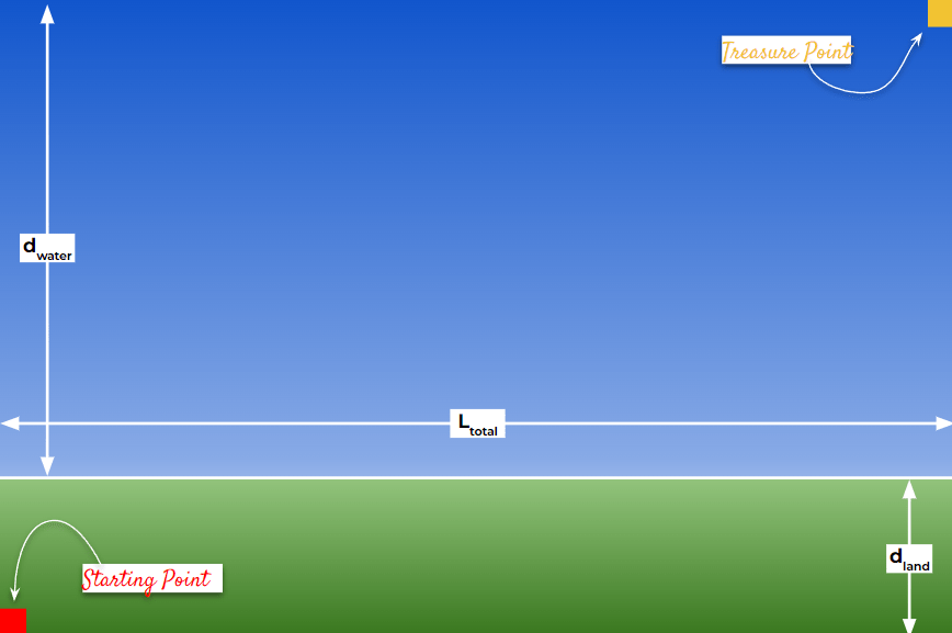
Imagine you’re standing on the bank of a wide field that leads straight into a serene lake, lets call that the Starting Point. Your goal: reach a Treasure Point diagonally across this combined stretch of land and water as fast as possible. You start at one corner on the land side and need to get to the opposite corner on the far side of the lake. You can run comfortably on land, and let’s say your running speed is pretty good—like how a hardworking aspiring student dashes to catch the last bus home after attending the preparation classes. But once you get into the water, the story changes. In the lake, you cannot hope to maintain that same pace—your swimming speed is slower.

Now, think carefully: Where should you enter the water for the fastest overall journey? Should you jump into the lake early, reducing land distance but increasing water distance? Or should you run along the land for a longer stretch, so that by the time you dive in, your watery crossing is shorter?

This isn’t a trivial problem—take a pause, picture the scenario in your mind. If you just pick a spot blindly, you might end up with a longer total time than if you’d chosen more wisely and you are NOT the only one who eyes the treasure. Here is your time to take your time and think!

Why is this Puzzle Interesting?

Because it’s a puzzle that looks simple on the surface but has few layers of complexity underneath. At its core this simply a distance and speed problem with a tint of calculus infused in it. Well, the last part is NOT even needed for throwing a guess. Need a hint? Think Maxima Minima Formulation. But for a seasoned eye, even that is NOT needed. So do you have an answer already? Awesome, let’s try to formulate the problem together. Take your hint at any stage and solve further.

Problem Formulation.

Now let’s bring some mathematics into play. We know:

• v_land ​: your speed on land.
• v_water ​: your speed in water.
• d_land ​: the width of the land strip you must cross.
• d_water ​: the width of the water body.
• L : the total horizontal distance along the length.

And to further assist us in the formulation, let us define the origin of the cartesian plane at the starting point.

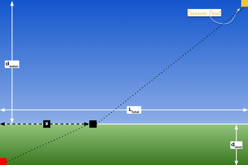
• Let d_land​ be the vertical width of the land region. That means you start at (0,0) and must first cross up to (0, d_land) at least vertically.
• Let d_water be the vertical width of the water region that follows. So, the total vertical distance from start to finish is d_land + d_water​.
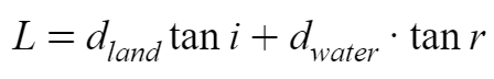
• Let L be the total horizontal length of the rectangle. You start on the left side at (0,0) and want to end at the far right corner at (L, d_land + d_water).

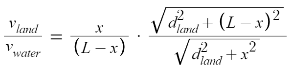
The only deciding factor remains at what horizontal point ‘x’ should you leave the land and plunge into the water? If at the point where you enter the water’s edge the horizontal coordinate is x, that means you have run diagonally across the land from (0,0) to (x, d_land), and then you will swim diagonally from (x, d_land) to (L, d_land + d_water).

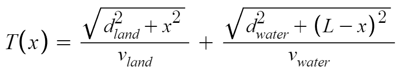
Given the speeds on land and water one can easily formulate the total time required to reach the treasure point. The total time T(x) to reach the end can be expressed as,

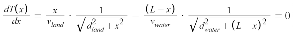
This is a function of x. To find the value of x that makes T(x) minimum (which means the fastest route), one must use the concepts of maxima and minima from calculus. You take the derivative T′(x) and set it equal to zero.

This equation can be simplified and rearranged, but it generally results in an implicit equation that is a little difficult to solve analytically, but it is definitely possible.

The Revelation.

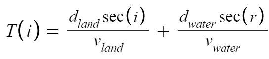
So far we have treated this problem as fundamentally a mathematical problem. Which is indeed correct formulation of the puzzle statement. But here comes the twist in the game. Everything remains same but instead of using x as the variable, now lets try to take the angle of exit from the land as the variable and formulate the problem around it. We will call that angle, i.

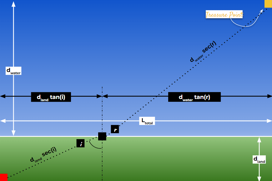
In this formulation, the total time required to reach the treasure point, T(i), can be expressed as,

Now to minimize T(i) wrt i we need to differentiate and equate to zero as done earlier,

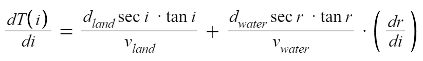
One needs to identify dr/di. Which can be easily evaluated using the following relationship,

And then differentiating it to unveil dr/di,

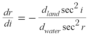
Upon substituting and restructuring it, the gist of the problem reveal itself in front of us, and here it is,

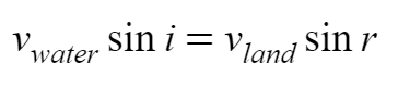
Does this result look any familiar to you? At least for once in your life you must have seen this equation in early science classes in your childhood. Well, this brings my childhood in front of me undoubtedly.

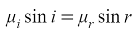
This is reminiscent of Snell’s Law in optics, where light traveling from one medium to another changes its direction to minimize travel time. Here, velocities​ play roles analogous to the inverse of refractive indices. If it hard for you to recall, here is Snell’s Law from Optics,

The exact final equation still won’t be trivially solvable, but the analogy gives you a beautiful insight: The best path to take when transitioning from fast land-travel to slow water-swimming follows the same principle that light uses when passing through different media at different speeds. It’s a powerful connection—your running and swimming path mimics how nature itself optimizes travel times for light rays.

Finding the Solution.

To really get the final answer, we turn to numerical methods. Python’s fsolve function from the scipy.optimize library is a tool that can tackle such equations. You plug in the equation, provide a guess, and let the computer do the heavy lifting because we are going to be busy handling the treasure gold. Here is the Python Code used to solve the implicit equation numerically and find the solution to the Puzzle.

import numpy as np
import matplotlib.pyplot as plt
from ipywidgets import interact, FloatSlider, interactive, Layout
from scipy.optimize import fsolve

# This function visualizes the path optimization problem where a person must travel across land and then water.
# The objective is to determine the angle at which the person should enter the water to minimize total travel time.
def visualize_landWater_problem(d1=1, d2=3, l=10, vLand=1, vWater=0.5):

    # Define the function for the implicit equation based on the incident angle "i"
    # This equation is derived from setting up the time minimization condition.
    # i: incident angle, d1: land width, d2: water width, l: total horizontal length, vL: speed on land, vW: speed in water
    def func_incidentAngle(i, d1, d2, l, vL, vW):
        # Returns the value of the function that needs to be zero for the correct angle.
        # The equation is constructed from Snell's Law-like conditions and time minimization.
        return d2 * vW * np.sin(i) / np.sqrt(vL**2 - (vW * np.sin(i))**2) - l + d1 * np.tan(i)

    # Plot the rectangular scenario:
    # Bottom line, top line, left vertical, right vertical boundaries
    plt.plot([0, l], [0, 0], linestyle='-', color='black')             # Bottom boundary
    plt.plot([0, l], [d1 + d2, d1 + d2], linestyle='-', color='black') # Top boundary
    plt.plot([0, 0], [0, d1 + d2], linestyle='-', color='black')       # Left boundary
    plt.plot([l, l], [0, d1 + d2], linestyle='-', color='black')       # Right boundary

    # Set plot limits
    plt.xlim([0, l])
    plt.ylim([0, d1 + d2])

    # Marking starting point (P1) and ending point (P2)
    plt.text(-(d1 + d2) / 5, -(d1 + d2) / 5, 'P1: Starting Point')
    plt.text(l + (d1 + d2) / 10, 6 * (d1 + d2) / 6, 'P2: Ending Point')

    # Draw the line separating land and water
    plt.plot([0, l], [d1, d1], linestyle='--', color='black')

    # Solve for the incident angle using fsolve
    soln_incidentAngle = fsolve(func_incidentAngle, 1, args=(d1, d2, l, vLand, vWater))[0]

    # Depending on the relative speeds, calculate the refraction angle
    if vWater < vLand:
        soln_refractionAngle = np.arcsin(vWater * np.sin(soln_incidentAngle) / vLand)
    else:
        soln_refractionAngle = np.arcsin(vLand * np.sin(soln_incidentAngle) / vWater)

    # Print the solutions for angles in degrees
    print(f'Solution: i = {soln_incidentAngle * 180 / np.pi:.2f} degree')
    print(f'Solution: r = {soln_refractionAngle * 180 / np.pi:.2f} degree')

    # Plot the optimal path lines:
    # From P1 to entry point in water (diagonal on land)
    plt.plot([0, d1 * np.tan(soln_incidentAngle)], [0, d1], color='brown')
    # Draw a dashed line upwards from the entry point for visual reference
    plt.plot([d1 * np.tan(soln_incidentAngle), d1 * np.tan(soln_incidentAngle)], [0, l], color='black', linestyle='--')
    # From water entry point to P2 (diagonal in water)
    plt.plot([d1 * np.tan(soln_incidentAngle), l], [d1, d1 + d2], color='tab:blue')

    # Shade regions to distinguish water and land visually
    plt.fill_between([0, l], [d1 + d2, d1 + d2], color="tab:blue", alpha=0.3)
    plt.fill_between([0, l], [d1, d1], color="brown", alpha=0.5)

    # Calculate and print the speed ratio and total time for the chosen path
    print(f'\nSpeed Ratio = {vLand / vWater:.2f}')
    total_time = d1 / (vLand * np.cos(soln_incidentAngle)) + d2 / (vWater * np.cos(soln_refractionAngle))
    print(f'Total Time (s)= {total_time:.2f} sec')

    # Set equal aspect ratio for a neat visualization
    ax = plt.gca()
    ax.set_aspect('equal', adjustable='box')


# Set up slider layout and create interactive sliders
slider_layout = Layout(width='500px', description_width='initial')

d1_slider = FloatSlider(min=0.1, max=5.0, step=0.1, value=2, description="Land Width (m)", layout=slider_layout)
d2_slider = FloatSlider(min=0.1, max=5.0, step=0.1, value=5, description="Water Width (m)", layout=slider_layout)
l_slider = FloatSlider(min=0.1, max=10, step=1, value=10, description="Length (m)", layout=slider_layout)
vLand_slider = FloatSlider(min=0.1, max=5.0, step=0.01, value=2, description="Speed on Land (m/s)", layout=slider_layout)
vWater_slider = FloatSlider(min=0.1, max=5.0, step=0.01, value=1, description="Speed in Water (m/s)", layout=slider_layout)

# Function to update the max water speed based on the current land speed
def update_v_water_range(*args):
    vWater_slider.max = vLand_slider.value

# Observe changes in land speed to adjust water speed range dynamically
vLand_slider.observe(update_v_water_range, 'value')

# Create an interactive UI that updates the plot based on slider values
ui = interactive(visualize_landWater_problem, d1=d1_slider, d2=d2_slider, l=l_slider, vLand=vLand_slider, vWater=vWater_slider)
display(ui)

But, Why Bother?

By experimenting with different values of v_land and v_water​, you’ll see how the optimal path changes. Just like light bends more sharply if there’s a bigger difference in refractive indices, you’ll find your optimal entry point into the water changes if there’s a bigger difference in your running and swimming speeds. It’s a mesmerizing sight: a non-obvious math puzzle unexpectedly mirroring the behavior of light beams!

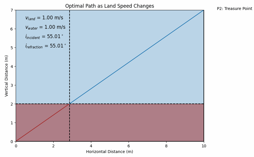
Do you wish to take some time and consider some corner cases: What if your swimming speed equals your running speed? What if the water is extremely shallow or the distances are huge? By experimenting with the code, you’ll uncover how the solution behaves under different conditions.

By shifting from the “where do I jump in?” (distance-based) approach to the “at what angle do I approach?” (angle-based) approach, we haven’t necessarily made the math simpler. We still have an equation that we can solve only numerically. But we’ve gained a conceptual lens that makes the problem feel more elegant and familiar. Instead of a random optimization problem, we see a deep parallel with a well-studied physical phenomenon. That perspective can be a joy in itself—it’s always uplifting to discover hidden unity in different areas of science which we at NotRocketScience always try to bring up for YOU.

Even if the final equations remain complicated, the shift in perspective, and the connection to a fundamental physical law, leaves you with a smile. It’s like seeing the world in a new light—quite literally.

TL;DR.

Generated using AI

• Puzzle Overview: Determine the optimal entry point into water on a path that spans both land and water to minimize total travel time while transitioning from running to swimming.
• Complexity and Calculus: This seemingly simple problem involves calculating the most efficient path, incorporating principles similar to those used in Snell’s Law of optics, where light changes direction to minimize travel time across media with different properties.
• Solution Approach: The challenge involves using variables like speeds on land and water, and distances of land and water stretches. The optimal point or angle for water entry is determined mathematically, typically requiring numerical methods like Python’s fsolve.
• Connection to Physics: The problem is analogous to Snell’s Law, illustrating how the fastest path involves entering water at an angle that minimizes travel time, similar to light refraction.